Day 2 · Modeling, connectivity, and ICA

Day 2Session 2.4Kiehl1:30 hHands-on session

SPM GUI for single subjects: explore design, scaling, results

A hands-on session in which participants specify, estimate, and view results for a single-subject auditory oddball model in the SPM GUI, using the course cheat sheet. The lecture component explains the types of intensity scaling in SPM, session (mean) scaling versus proportional (global) scaling, and why proportional scaling can produce both false positives and false negatives when the global signal correlates with the task.

Take-aways

  • Session scaling removes between-run mean differences and is standard; proportional scaling divides by the global mean and is risky.
  • If the global signal correlates with the task, proportional scaling creates false deactivations and hides true activations; leave global normalisation at none.
  • In SPM the design is built from onsets per condition and run, estimated from SPM.mat, and tested with contrast vectors that must match the column order including derivatives and block effects.

Key terms

  • session scaling
  • proportional scaling
  • global brain mean
  • adjusted proportional scaling
  • Type I and Type II errors
  • fMRI model specification
  • microtime resolution
  • temporal derivative
  • contrast manager
  • Check Reg
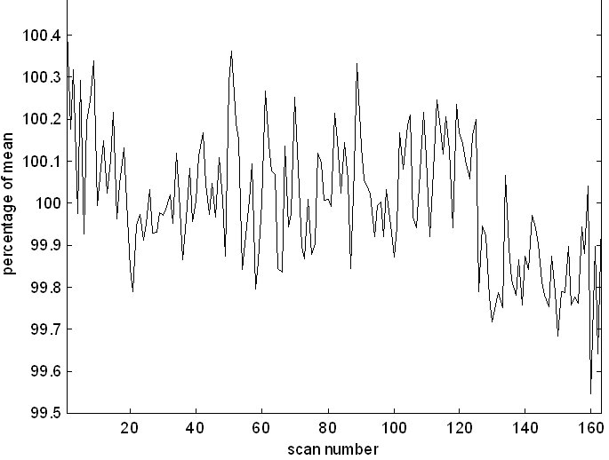
Global mean signal across scans before adjustment
Global mean signal across scans before adjustment. Lecture 2.4 slides (Kiehl)

Outline

What the session covers

01Session (mean intensity) scaling

  • Also called global mean scaling, block effect, or mean intensity scaling.
  • Purpose: remove intensity differences between runs, i.e., differences in the mean of the whole time series.
  • Runs can have different mean values, so between-run variance must be compensated for.
  • Each run is usually scaled to a mean of 100 (or 50 or similar).

02Proportional (global) scaling and its dangers

  • Proportional scaling divides each scan's intensities by that scan's mean over all voxels (the global brain mean).
  • Intended to remove global drifts and improve sensitivity.
  • The global mean must be independent of task activity; if it correlates with the task, scaling can dramatically change the results.
  • A voxel of no interest divided by a task-correlated global signal appears negatively correlated with the task: a false deactivation (Type I error).
  • A task-related voxel divided by a task-correlated global signal becomes nearly flat and is missed (Type II error).
  • In the SPM batch, global normalisation should be left at 'none'; do not click 'scale'.
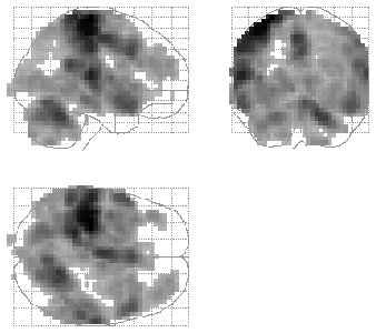
Glass-brain map showing widespread global-signal-related effects
Glass-brain map showing widespread global-signal-related effects. Lecture 2.4 slides (Kiehl)
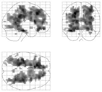
SPM glass-brain projection of a thresholded statistical map
SPM glass-brain projection of a thresholded statistical map. Lecture 2.4 slides (Kiehl)

03Evidence: adjusted proportional scaling in an oddball study

  • Desjardins, Kiehl and Liddle (2001) compared no scaling, proportional scaling, and adjusted proportional scaling (global signal orthogonalized to the covariates of interest).
  • For target responses, proportional scaling produced considerably fewer activations; no scaling and adjusted scaling looked similar.
  • Z-scores were highest with adjusted scaling and lowest with proportional scaling, e.g., SMA: 12.79 (none), 10.39 (proportional), 13.17 (adjusted).
  • Novel-stimulus activations were similar across methods, consistent with a low correlation between the global signal and the novel covariate.
  • The component removed by orthogonalization was small: global signal SD 0.157% of mean, difference between global and adjusted global 0.0328%.
  • Further reading: Macey et al. 2004, Aguirre et al. 1998, Andersson 1997, Andersson et al. 2001.

04Specifying and estimating the single-subject model in SPM

  • Data: subject s01 of the auditory oddball dataset, two runs of 189 smoothed, warped volumes (sws01_aod_run1.nii, sws01_aod_run2.nii).
  • Timing parameters: units in scans, interscan interval 2, microtime resolution 30, microtime onset 15.
  • Three conditions per run (targets, novels, standards) with onsets loaded via spm_load from the s01\beh text files and duration 0.
  • Basis functions: canonical HRF with time derivatives; global normalisation none; serial correlations none.
  • Contrast columns per run are target, target derivative, novel, novel derivative, standard, standard derivative, followed by two block effects.
  • Use Check Reg with mask.img and a canonical T1 to confirm the analysis mask looks reasonable.
PINES negative-affect signature rendered on cortical surfaces — Chang et al. (2015), PLoS Biology

Hands-on

Step by step

The walk-through below is distilled from the course cheat sheets. Data paths refer to the course Dropbox folder (e.g. data/auditory_oddball).

  1. Open SPM, fMRI model specification; set Directory to c:\mind\data\auditory_oddball\AOD_raw\s01\stats.
  2. Timing parameters: Units for design = scans; Interscan interval = 2; Microtime resolution = 30; Microtime onset = 15.
  3. Data & Design: add two subject/sessions. For run 1, select sws01_aod_run1.nii frames 1-189 using filter 'sw.*' and frames [1:200]; right-click and 'select all'.
  4. Add three conditions for run 1: targets (onsets via spm_load from s01\beh\targets_run1.txt), novels (novels_run1.txt), standards (nontargs_run1.txt); Durations = 0; leave time and parametric modulations empty.
  5. Repeat for run 2 with sws01_aod_run2.nii and the run2 onset files.
  6. Basis functions: canonical HRF; Model derivatives = time derivatives. Leave Volterra interactions off.
  7. Global normalisation = none (never 'scale'); Explicit mask empty; Serial correlations = none. Run the batch.
  8. Press Estimate and select SPM.mat in the s01\stats directory.
  9. Press Results, select SPM.mat, and define the contrast targets vs. standards. With derivatives: .5 0 0 0 -.5 0 .5 0 0 0 -.5 0 (per run: target, target deriv, novel, novel deriv, standard, standard deriv; then two block effects).
  10. If derivatives were not modelled, use .5 0 -.5 .5 0 -.5 0 0 (target, novel, standard per run, then two block effects).
  11. Inspect the thresholded results and outputs written to s01\stats.
  12. Use Check Reg to overlay mask.img on a t1.img from SPM's canonical folder and confirm the mask covers the brain.
Cheat sheet: fMRI model specification — full cheat sheet

Mind fMRI Image Acquisition and Analyses Course - Cheat Sheet for Course Stats Processing.

-fMRI model specification

- Directory – ‘select c:\mind\data\auditory_oddball\AOD_raw\s01\stats’

- Timing parameters –

Units for design - select ‘scans’

Interscan interval - enter ‘2’

Microtime resolution – enter ‘30’

Microtime onset – enter ‘15’

-Data & Design <-X *click twice and add two subject/sessions

+ subject/session

Scans – enter all the ‘sw*.nii’ scans (smoothed/warped) for s01\run1\sw* - use the filter settings ‘sw.*’ in the window to help you select the right scans also use the filter settings [1:200] in the window to help you select the right scans Right click on mouse and ‘select all’ images sws01_aod_run1.nii,1 to sws01_aod_run1.nii,189’)

Conditions *click three times to add three conditions

Name – ‘targets’

Onsets – spm_load – then select s01\beh\targets_run1.txt

Durations -‘0’

Time modulations

Parametric modulations

Condition (double click to highlight)

Name ‘novels’

Onsets – spm_load – then select s01\beh\novels_run1.txt

Durations -‘0’

Time modulations

Parametric modulations

Condition (double click to highlight)

Name ‘standards’

Onsets – spm_load – then select s01\beh\nontargs_run1.txt

Durations -‘0’

Time modulations

Parametric modulations

Multiple conditions

Regressors

Multiple regressors

High-pass filter

+Subject/session

Scans – enter all the ‘sw*.nii’ scans (smoothed/warped) for s01\run2\sw* - use the filter settings ‘sw.*’ in the window to help you select the right scans also use the filter settings [1:200] in the window to help you select the right scans Right click on mouse and ‘select all’ images sws01_aod_run2.nii,1 to sws01_aod_run2.nii,189’)

Conditions *click three times to add three conditions

Name – ‘targets’

Onsets – spm_load – then select s01\beh\targets_run2.txt

Durations -‘0’

Time modulations

Parametric modulations

Condition (double click to highlight)

Name ‘novels’

Onsets – spm_load – then select s01\beh\novels_run2.txt

Durations -‘0’

Time modulations

Parametric modulations

Condition (double click to highlight)

Name ‘standards’

Onsets – spm_load – then select s01\beh\nontargs_run2.txt

Durations -‘0’

Time modulations

Parametric modulations

Multiple conditions

Regressors

Multiple regressors

High-pass filter

Factorial design

Basis functions *click on this to expand

-canonical HRF

Model derivatives - select ‘time derivatives’

Model interactions (volterra)

Global normalization (none) *** recall we never want to accidently click ‘scale’ here – a big NO NO!

Explicit Mask

Serial Correlations *click to expand

- Select None.

Contrasts. So once you have modelled the data and also run thru the ‘Estimate’ button, selecting the SPM.mat file in the stats directory you are ready to hit the ‘Results’ button and specify a contrast.

A simple contrast you can specify is Targets vs Nontargets (Standards) and assuming you included the temporal derivative, this is the contrast for this: .5 0 0 0 -.5 0 .5 0 0 0 -.5 0 (run 1) target, target derivative, novel, novel derivative, standard, standard derivative, (run 2) target, target derivative, novel, novel derivative, standard, standard derivative, block effect, block effect) You can copy and paste this contrast in the contrast manager.

If you did not model the temporal derivative, then use this contrast for targets vs standards.

.5 0 -.5 .5 0 -.5 0 0 (target, novel, standard, target, novel, standard, block effect, block effect).

Outputs are placed in the s01/stats directory. Always make sure to use ‘check reg’ and select the mask.img and a t1.img (from the canonical folder in spm) to see if your mask looks ok.

From the instructors' research

Related figures

Examples of these concepts in published work by the course instructors.

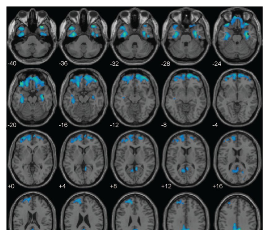
Paralimbic gray matter reductions associated with psychopathy
Paralimbic gray matter reductions associated with psychopathy. Ermer et al. (2012), Journal of Abnormal Psychology
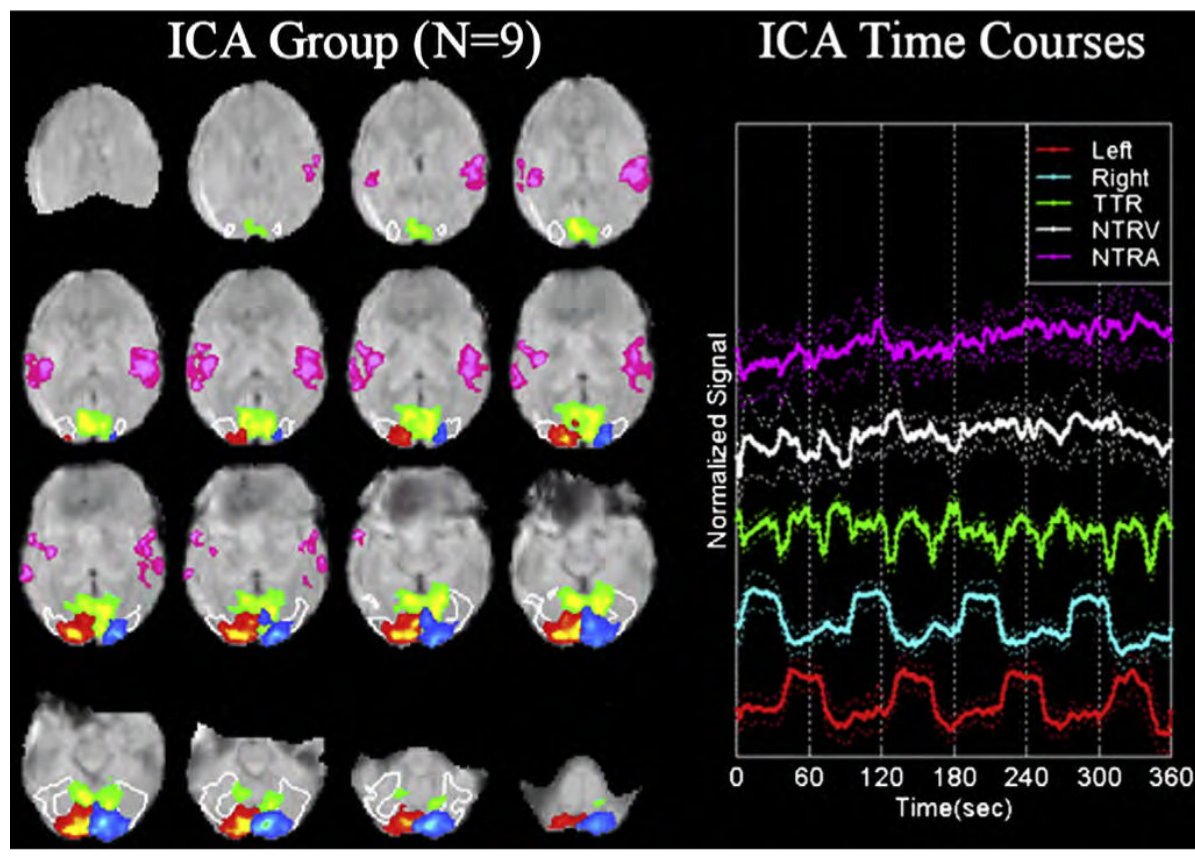
Group ICA component maps and their task-related time courses
Group ICA component maps and their task-related time courses. Calhoun et al. (2009), NeuroImage