Basis sets: flexible hemodynamic modeling

This session explains why a single canonical HRF is often wrong for a given voxel, region, or population, and how temporal basis sets (canonical plus derivatives, finite impulse response) let the GLM fit a range of response shapes. It covers how to recover interpretable amplitude, time-to-peak, and width estimates from flexible fits, and frames basis-set choice as a bias-variance trade-off that depends on the task and brain region.

Scroll down

Take-aways

A fixed canonical HRF is usually wrong somewhere in the brain or population, and mis-modeling can create or hide amplitude differences.
Basis sets make the HRF shape a linear estimation problem; more flexibility improves accuracy at the cost of precision and interpretability.
Use tools such as spm_htw_from_fit to convert flexible fits into amplitude, timing, and width images that can be taken to group analysis.

Key terms

canonical HRF
temporal basis function
time and dispersion derivatives (SPM-3)
finite impulse response (FIR)
deconvolution
bias-variance trade-off
amplitude, time-to-peak, width
spm_htw_from_fit
HRF mis-modeling

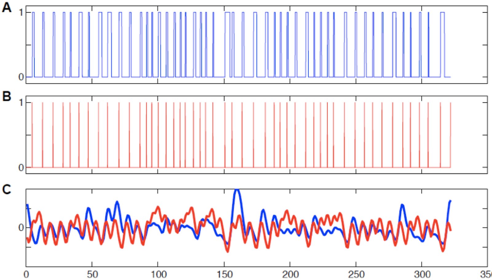
**Variable-duration versus constant-impulse models and their convolved predictors.** Lecture 2.5 slides (Wager)

Outline

What the session covers

01Review: neural event models and the canonical HRF

Multiple predictors are built by convolving each condition's indicator function with an HRF.
The choice between events and epochs matters more than expected, e.g., modeling trial-to-trial reaction time with mean RT around 1 s (Grinband et al. 2008).
The canonical HRF is a linear combination of two gamma functions; optimal if correct, but biased with lower power if wrong.
The same HRF is unlikely to hold for all voxels: responses may be faster or slower, have different undershoots, or peak later.
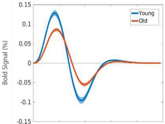
Aging reduces HRF amplitude and disperses its shape; dementia and pharmacological states also change the HRF.

02Temporal basis functions

Model the HRF as a linear combination of pre-specified functions f_i(t); the stimulus function is convolved with each basis to form a set of predictors.
Parameter estimates are weights on the basis functions, giving the weighted sum that best fits the response.
Fit separately for each trial type in each voxel for each person; the design matrix has one predictor per condition per basis function.
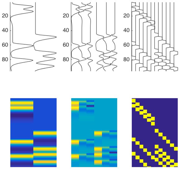
Three common sets: canonical HRF (one parameter), HRF plus time and dispersion derivatives ('SPM-3'), and finite impulse response (one column per time point).
Basis sets differ in how much they assume a priori about shape and which HRF shapes they can capture.
HRF shape varies across regions: lateral occipital peaks at 6-8 s, hippocampus at 10 s with a response at 16 s (Summerfield 2006).

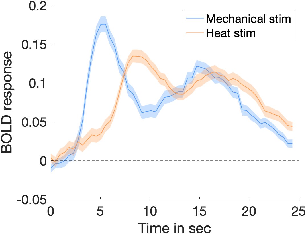
**Basis-set fits of BOLD responses to mechanical versus heat stimulation.** Lecture 2.5 slides (Wager)

**Basis functions and the design matrices they generate.** Lecture 2.5 slides (Wager)

03Flexible fits and neural versus vascular sources

The observed response depends on both the neural activity time course and vascular hemodynamics; these are hard to separate.
The overall estimated HRF captures the joint neural and hemodynamic effect and is robust to neural-model misspecification within the limits of the basis set.
With an inflexible model, a change in response duration can be mistaken for a change in amplitude (Lindquist 2007, 2009; Waugh 2010).

04Estimating amplitude, timing, and width from fits

CanlabCore function spm_htw_from_fit.m: run it in the SPM first-level directory, ideally after specifying contrasts.
Outputs per condition: htw_amplitude_001.nii, htw_time_to_peak_001.nii, htw_width_001.nii, htw_area_under_curve_001.nii.
Contrast images across conditions are named from SPM.xCon.name, e.g., con_htw_ampl_targetvsstandards5.nii, con_htw_time_..., con_htw_widt_..., con_htw_area_....
Take these to second-level group analysis, with separate analyses for amplitude, time, and width.

**Hemodynamic response shapes for young and older adults.** Lecture 2.5 slides (Wager)

05Choosing a basis set

Accuracy: can the model capture the true response without systematic bias? Precision: are parameters estimated with little error variance?
This is the bias-variance trade-off; more flexible sets are more accurate but less precise.
Prefer few parameters (precision), parameters that are interpretable (e.g., amplitude), and accuracy in the physiological range that matters for your task and region.
The three-parameter set captures a limited family of curves, suits events or short epochs, and needs amplitude estimation not built into SPM or FSL.
Often three parameters are not enough: aging dispersion is not corrected, and sustained responses (e.g., to aversive images) appear as lower or reversed amplitude.
FIR fits for each stimulus type reveal shape and duration differences that fixed-shape models miss; see Lindquist and Wager 2007 and Lindquist et al. 2009.

Five dynamic connectivity states rendered on cortical surfaces — Rashid et al. (2014), Frontiers in Human Neuroscience

Previous · 2.4SPM GUI for single subjects: explore design, scaling, results Next · 2.6Derivative boost

Day 2 · Modeling, connectivity, and ICA

2.1 GLM model building: predictors and contrasts 2.2 GLM filtering and nuisance regressors 2.3 GLM multicollinearity and diagnostics 2.4 SPM GUI for single subjects: explore design, scaling, results2.5 Basis sets: flexible hemodynamic modeling2.6 Derivative boost 2.7 Parametric modulators 2.8 Autocorrelation and generalized linear models 2.9 Intro to connectivity and mediation; mediation demo/walkthrough 2.10 Introduction to ICA: Independent Component Analysis