fMRI physics, pulse sequences, and reconstruction

Covers the physics needed to understand an fMRI dataset: nuclear spin and the Larmor equation, T1 and T2 relaxation, spin and gradient echoes, spatial encoding with gradients and k-space, and echo-planar imaging. Then explains the BOLD contrast mechanism, susceptibility artifacts and how to reduce them, and the practical trade-offs among TR, TE, flip angle, slices, bandwidth, matrix, and field of view.

Scroll down

Take-aways

BOLD is a T2* effect: less deoxyhemoglobin means a more uniform field and more gradient-echo EPI signal, but the change is only a few percent.
Susceptibility near air-tissue interfaces causes both signal loss and geometric distortion, mostly along the phase-encode direction; shorter encoding time and parallel imaging help.
Every EPI parameter trades SNR against speed, coverage, and artifact; a TR of 1 to 2 s, TE near 30 ms at 3 T, flip angle 60 to 70 degrees, and isotropic voxels are sensible defaults.

Key terms

Larmor frequency
T1 and T2 relaxation
T2*
spin echo vs. gradient echo
k-space
echo-planar imaging (EPI)
BOLD contrast
susceptibility
phase-encode direction
Ernst angle

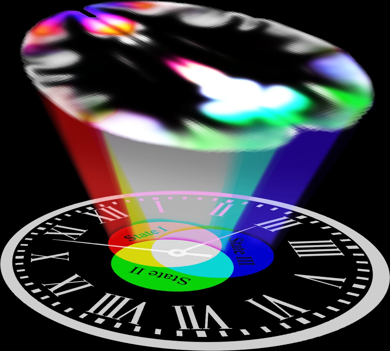
**Phase-clock rendering of MR signal states.** Lecture 1.2 slides (Calhoun)

Outline

What the session covers

01MR basic principles: spin and relaxation

Protons have spin and precess at the Larmor frequency, omega = gamma times B0; gamma is 42 MHz/T for protons (11 MHz/T for carbon-13).
An RF pulse tips magnetization by 90 or 180 degrees; the signal decays and recovers afterward.
T1 (longitudinal, spin-lattice) relaxation is recovery of magnetization along B0; T2 (transverse, spin-spin) is decay of the measurable signal.
Relaxation times are tissue specific: T1 about 600 ms (white matter), 1000 ms (gray), 3000 ms (CSF); T2 about 70, 90, and 400 ms.
T2 is much shorter than T1; 200 ms after the pulse about 5 percent (white), 10 percent (gray), and 60 percent (CSF) remains.

02Contrast and echoes

TR and TE set contrast: long TR/short TE gives proton density, short TR/short TE gives T1, long TR/long TE gives T2.
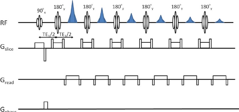
A spin echo uses a 90 then 180 degree pulse to refocus dephasing (Hahn echo; CPMG for multiple echoes) and measures T2.
A gradient echo does not refocus static field inhomogeneities, so it measures T2*; this sensitivity is what BOLD fMRI relies on.

**Spin-echo pulse sequence timing diagram.** Lecture 1.2 slides (Calhoun)

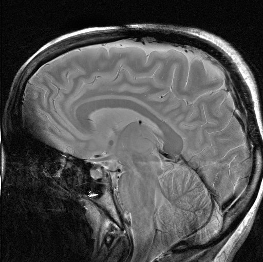
**Sagittal T2-weighted structural MRI slice.** Lecture 1.2 slides (Calhoun)

03Making an image: gradients, k-space, EPI

Slice selection: a gradient makes field strength depend on z (B = B0 + Gz z), so only one slab resonates with the RF pulse.
Frequency encoding along x makes precession rate depend on position; phase encoding along y uses a brief gradient stepped up on each repeat.
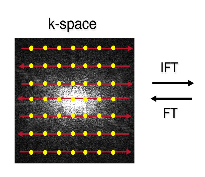
The raw data matrix (k-space) fills line by line with each phase-encode step; a 2D Fourier transform yields the image.
EPI and spirals both cover k-space in one shot: EPI gives distortion and ghosts, spirals give blurring; spirals sample k = 0 first.
In an EPI image, x corresponds to frequency and y to phase encoding, which matters for where distortion appears.

04Basics of BOLD fMRI

Hemodynamic measures of brain function date to Mosso (1881), who saw regional cortical pulsation change with mental activity.
BOLD chain: neural activity up, blood flow up (reactive hyperemia), deoxyhemoglobin down, field homogeneity up, gradient-echo EPI signal up.
Two-photon imaging in mice shows arterial dilation following neural activity after whisker stimulation (Chow et al., 2020).
Signal changes are small, 0.5 to 3 percent at 1.5 T, invisible in a single image; we always analyze differences or time courses.
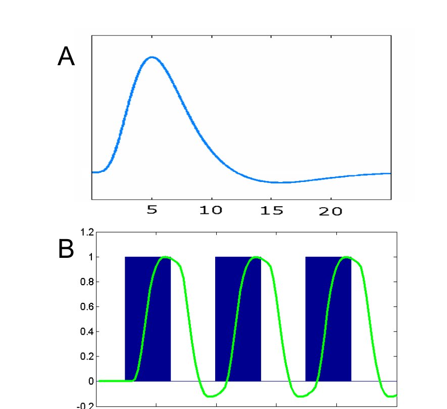
The response is delayed and slow (about 10 s), so even short events produce a long response.
A typical volume is 64 x 64 voxels x 25 slices, about 102,400 voxels.

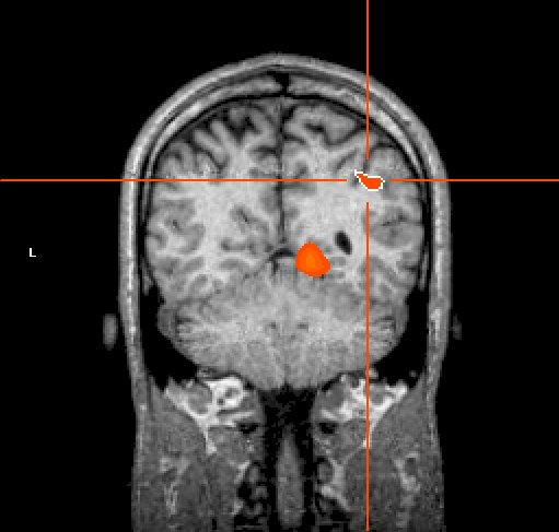
**Coronal MRI with focal activation cluster.** Lecture 1.2 slides (Calhoun)

05Susceptibility: the good, the bad, the ugly

Deoxyhemoglobin is paramagnetic (the good); air-tissue interfaces near sinuses and ear canals distort the field (the bad); fillings and implants are the ugly.
All susceptibility effects grow with B0.
Two consequences: through-plane dephasing causes signal loss within a voxel; in-plane gradients cause geometric distortion, mostly in the phase-encode direction.
EPI bandwidth is asymmetric, so distortion is about 100 times larger in the phase-encode direction; reversing the k-space traversal flips compression to expansion.
Shorter encoding time (e.g., 34 down to 17 ms) reduces distortion; parallel imaging (PAT/GRAPPA) shortens it further.
Other remedies: first and second order shimming, thinner slices, shorter TE, z-shim, tailored RF pulses, a mouth shim, field-map correction, multi-shot sequences, tilting slices.

06Choosing single-shot gradient-echo EPI parameters

TR: long TR maximizes raw SNR, but noise is physiologic and more time points help statistics; use a short TR, 1 to 2 s is reasonable.
Flip angle: the Ernst angle is 90 degrees for TR over 3 s and 60 to 70 degrees for TR 1 to 2 s; wrong angles cause inflow artifacts.
Slices: collect as many as fit in the TR; whole-brain coverage normalizes better and motion correction works best with thin slices.
Voxel size = FOV/matrix (200 mm/64 = 3.125 mm); SNR scales with voxel volume, but thin isotropic voxels reduce partial volume and dephasing.
TE: the optimum is shorter at higher field (about 30 ms at 3 T, 50 ms at 1.5 T); shorter TE trades BOLD contrast for less dropout.
Bandwidth of 128 kHz over a 64 matrix gives 2000 Hz per pixel; higher bandwidth means faster acquisition, more slices, less blur, more noise.

MRI scanner suite with patient table — Lecture 1.1 slides (Kiehl)

From the instructors' research