Day 1 · Acquisition, preprocessing, and the GLM

Day 1Session 1.8Wager1:00 hLecture

General Linear Model I: principles and fMRI

Introduces the General Linear Model as the workhorse of fMRI analysis: the model, its assumptions, how parameters are estimated, and what leverage and influence mean for design and outliers. Then shows how fMRI predictors are built by convolving stimulus functions with a hemodynamic response function, how a two-level (within-subject, then group) analysis is organized, and which files SPM writes at each stage.

Take-aways

  • The GLM finds betas that minimize squared error; independence of errors is the assumption that matters most.
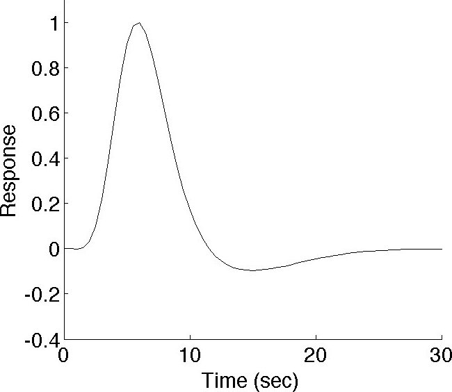
  • fMRI predictors are stimulus functions convolved with an HRF that peaks at 4 to 6 s and returns to baseline by 20 to 30 s.
  • Analyses are hierarchical: single-subject betas and contrasts (con images) feed a random-effects group test.

Key terms

  • General Linear Model
  • design matrix
  • beta (parameter estimate)
  • pseudoinverse
  • leverage and influence
  • hemodynamic response function (HRF)
  • convolution
  • linear time-invariant system
  • mass univariate
  • contrast image
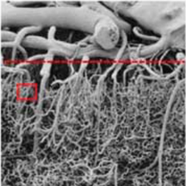
Micrograph of cortical vasculature
Micrograph of cortical vasculature. Lecture 1.8 slides (Wager)

Outline

What the session covers

01Framework: two-level strategy

  • Within-person questions: is the task effect greater than zero, or does brain activity track performance across trials?
  • Between-person questions: do task effects differ between groups or correlate with individual differences?
  • Level 1: fit a GLM in each voxel for each person and save summary statistics (betas, regression slopes).
  • Level 2: analyze those summary statistics across people (random effects) to determine what is significant at the population level.

02The GLM family and its assumptions

  • The GLM treats data as a linear combination of predictors plus noise; t-tests, ANOVA, ANCOVA, and OLS regression are all special cases.
  • Key assumption: errors are independent; violations invalidate the statistics. Normality and equal variance matter less.
  • The correlated-errors variant assumes a known dependence structure (repeated measures or time series), which is the fMRI situation.
  • Logistic regression is a GLM with a link function; a generalized inverse handles design matrices that are not full rank.
  • A decision flowchart maps predictor and outcome types to the classic named tests.
Canonical hemodynamic response function
Canonical hemodynamic response function. Lecture 1.8 slides (Wager)
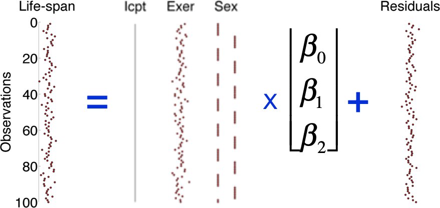
GLM schematic: data equals design matrix times betas
GLM schematic: data equals design matrix times betas. Lecture 1.8 slides (Wager)

03The model and how it is fit

  • y = X beta + epsilon: data equal design matrix times parameters plus residuals; predictors are known, parameters are estimated.
  • Predictors can be categorical (sex) or continuous (performance); the intercept is a column of ones.
  • Fitting minimizes the sum of squared residuals; beta = pinv(X) times y, geometrically a projection of y onto the space spanned by X.
  • Crime-rate versus police-expenditure example: a strong association, but beware causal inference when causes like urbanicity are unmodeled.
  • In MATLAB the whole fit is X = [i x]; b = pinv(X) * y; e = y - X*b.

04Leverage, influence, and power

  • Leverage is how far an observation's predictor values are from the predictor mean; high-leverage points can strongly affect the fit.
  • Influence is how much an observation actually changes the betas; it requires both high leverage and a large residual (Cook's distance).
  • An outlier at the mean of x has zero leverage and does not change the slope.
  • Design take-home: extreme x values create power; observations at the mean add little, which is why experiments beat observational correlations per observation.
  • Analysis take-home: check for predictors with uneven leverage and for influential outliers.
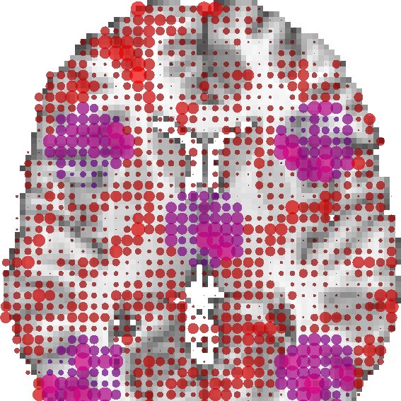
Voxel-wise effects across an axial brain slice
Voxel-wise effects across an axial brain slice. Lecture 1.8 slides (Wager)

05Building fMRI predictors: the HRF and convolution

  • Brief neural events produce a delayed, dispersed BOLD response; the HRF reflects blood oxygenation, flow, and volume (Buxton et al. 1998).
  • Empirical HRF: peak at 4 to 6 s, baseline by 20 to 30 s, sometimes an initial undershoot; similar in V1, A1, S1 but not necessarily elsewhere.
  • Vasodilation involves PGE2, COX-2, EETs, nitric oxide, and potassium; both glutamatergic and GABAergic transmission can drive it, and neuromodulators (ACh, NA, 5-HT, DA) shape it.
  • Linear time-invariant assumption: the predictor is the stimulus function (blocks or events) convolved with the HRF.
  • Each event type gets its own regressor (e.g., famous versus non-famous faces) and betas are compared with contrasts; factorial designs work the same way.
  • Assumptions to keep in mind: the neural activity function is right, the HRF is right, and the system is LTI.

06The GLM pipeline in SPM

  • SPM is mass univariate: the model is fit one voxel at a time to produce a statistical image.
  • Design specification is saved in SPM.mat; estimation writes beta_????.img and ResMS.img.
  • T-contrasts (c'b) write con_????.img and spmT_????.img; F-contrasts write ess.img and spmF_????.img.
  • Each participant's score is usually a contrast between conditions (e.g., task minus control) that goes to the group analysis.
  • Variance in the two-level model comes from unexplained error (E), design-related inefficiency (D), and individual differences (I).
Three axial slices with simulated effect patterns — Lecture 1.8 slides (Wager)

From the instructors' research

Related figures

Examples of these concepts in published work by the course instructors.

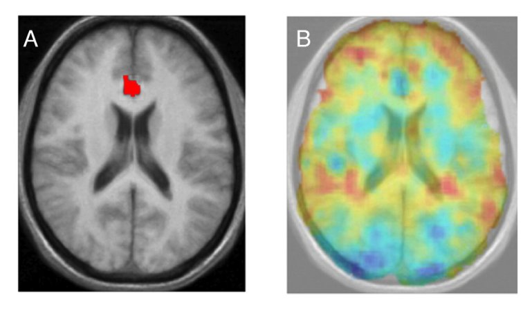
Region of interest and estimated HRF amplitude map
Region of interest and estimated HRF amplitude map. Lindquist et al. (2009), NeuroImage
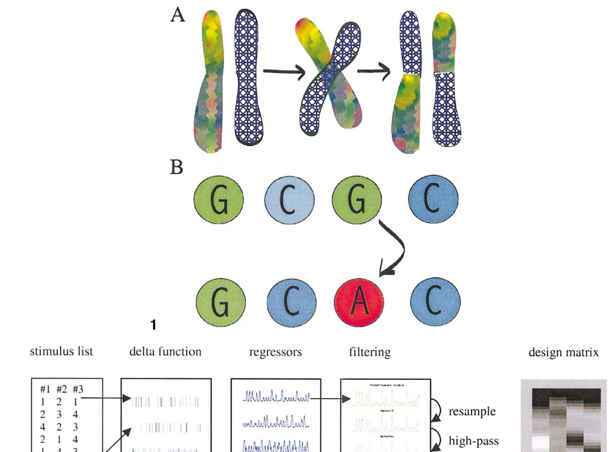
Genetic algorithm crossover and design-matrix construction for fMRI designs
Genetic algorithm crossover and design-matrix construction for fMRI designs. Wager & Nichols (2003), NeuroImage