Day 1 · Acquisition, preprocessing, and the GLM

Day 1Session 1.7Kiehl1:00 hHands-on session

Preprocessing: coregistration, normalization, smoothing

Covers moving each participant's data into a common stereotactic space so results can be compared across people, studies, and labs, and then smoothing the normalized images. Contrasts Talairach and MNI spaces, compares two normalization pathways (mean EPI to T1 to template versus mean EPI directly to the EPI template), and explains what spatial smoothing buys and costs. Hands-on: Old Normalize with the EPI template and 8 mm smoothing.

Scroll down

Take-aways

Report the space you actually used; MNI and Talairach differ by 10 to 15 percent and require conversion.
Normalizing the mean EPI directly to the EPI template handles EPI distortion that a linear coregistration to T1 cannot.
Smooth with a kernel of about 2 to 3 times the voxel size (8 mm here) to gain SNR and tolerance to anatomical variability, knowing that small activations will shrink.

Key terms

spatial normalization
Talairach space
MNI space
AC-PC line
EPI template
coregistration
nonlinear basis functions
reslicing / sinc interpolation
Gaussian kernel
FWHM

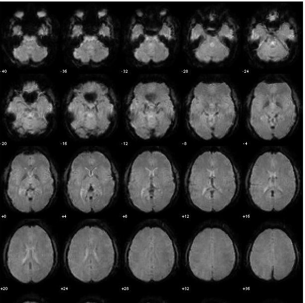
**Montage of normalized functional slices.** Lecture 1.7 slides (Kiehl)

Outline

What the session covers

01Why normalize, and into what space

Realignment aligns images within a person; normalization provides a mechanism for comparing data across labs and studies.
Talairach space: atlas by Talairach and Tournoux based on one French woman's brain; origin at the anterior commissure; oriented on the AC-PC line.
MNI space (adopted in SPM96): based on 304 normal subjects, more representative, and 10 to 15 percent larger than Talairach.
Much confusion in the literature; conversions between Talairach and MNI are needed for meta-analyses and ROI planning, and methods differ by group and software.
Manuscripts must state the actual space used.

02What an EPI volume looks like

Typical raw multiband EPI: 82 x 82 x 56 voxels at about 3 mm; after warping to MNI, 61 x 73 x 61 at 3 mm isotropic.
Non-uniform local fields cause through-plane dephasing: protons in different parts of a voxel drift out of phase by TE.
Dropout above the frontal sinus is worse for thick slices and at long TE (3 T examples from 21 to 60 ms).
EPI distortion appears as local compression or expansion depending on k-space direction; use the shortest possible encoding time.

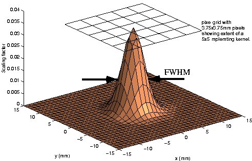
**3-D Gaussian smoothing kernel with FWHM.** Lecture 1.7 slides (Kiehl)

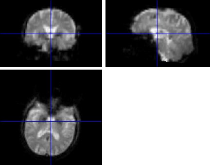
**Orthogonal views of a smoothed functional volume.** Lecture 1.7 slides (Kiehl)

03Two normalization pathways

Pathway A: coregister the mean EPI to the subject's T1, normalize the T1 to the T1 template, and apply those parameters to the EPI.
Problem with A: coregistration is a linear operation, so EPI warping and distortion are not accounted for unless you have field-map correction (which slows acquisition).
Pathway B: normalize the mean EPI directly to the EPI template; the nonlinear components account for EPI distortion (Calhoun et al. 2017, Human Brain Mapping).
Risk with B: if the mean EPI differs much from the EPI template, normalization can fail; tune the basis functions or build a site template.
Field-map correction improves either pathway when available.

04Reslicing and checking the output

Data must be resliced into MNI space with interpolation; sinc is likely best.
Choose the output voxel size: inputs were 3.44 x 3.44 x 5 mm; SPM's default is 2 mm isotropic; the course uses 3 mm.
Review the normalization postscript: it should report 4 x 5 x 4 basis functions; if 9 x 12 x 9, renormalize with nonlinear frequency cutoff 45.
Outputs: means01_aod_run1_sn.mat (native-to-MNI transform) and ws01_aod_run1.nii (warped images).

05Spatial smoothing

Smoothing increases signal-to-noise if the blur is smaller than the activation; cortical activations are larger than subcortical ones such as thalamus.
It compensates for imperfect spatial normalization and for functional anatomy that differs across people even when structure is aligned.
It facilitates inter-subject comparison, and smooth data is an assumption of the statistical model.
Cost: small activations are reduced; future thresholding strategies may reduce the need for smoothing.
Implementation: 3D convolution with a Gaussian; a fuzzy-edged ball replaces each voxel with a weighted average of its neighbors.
The class uses 8 x 8 x 8 mm FWHM; rule of thumb is 2 to 3 times the original voxel size.

MRI scanner suite with patient table — Lecture 1.1 slides (Kiehl)

Hands-on

Step by step

The walk-through below is distilled from the course cheat sheets. Data paths refer to the course Dropbox folder (e.g. data/auditory_oddball).

In the SPM GUI click Utils > cd and set the working directory to c:\mind.
Click Normalise; in the batch window delete the default Normalise module, then choose SPM > Tools > Old Normalise > Estimate & Write.
Expand Normalise: Estimate & Write, click Data, and click New Subject four times (2 subjects x 2 sessions).
For each Subject: Source Image = the mean EPI for that session (e.g., means01_aod_run1.nii); Images to Write = all frames s01_aod_run1.nii,1 to 189 (filter [1:200], Select All).
Under Estimation Options set Template Image to c:\mind\toolboxes\spm12\toolbox\OldNorm\EPI.nii; leave the rest at defaults.
Under Writing Options confirm the voxel size is 3 x 3 x 3 mm, then click Run.
Check the postscript output for 4 x 5 x 4 basis functions (if 9 x 12 x 9, rerun with nonlinear frequency cutoff = 45) and confirm *_sn.mat and ws01_aod_run1.nii files exist.
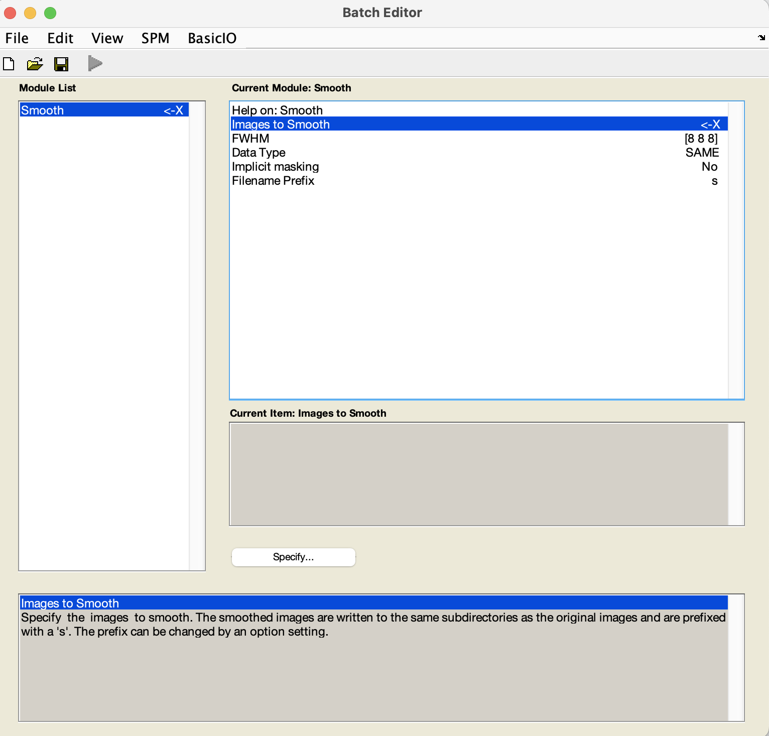
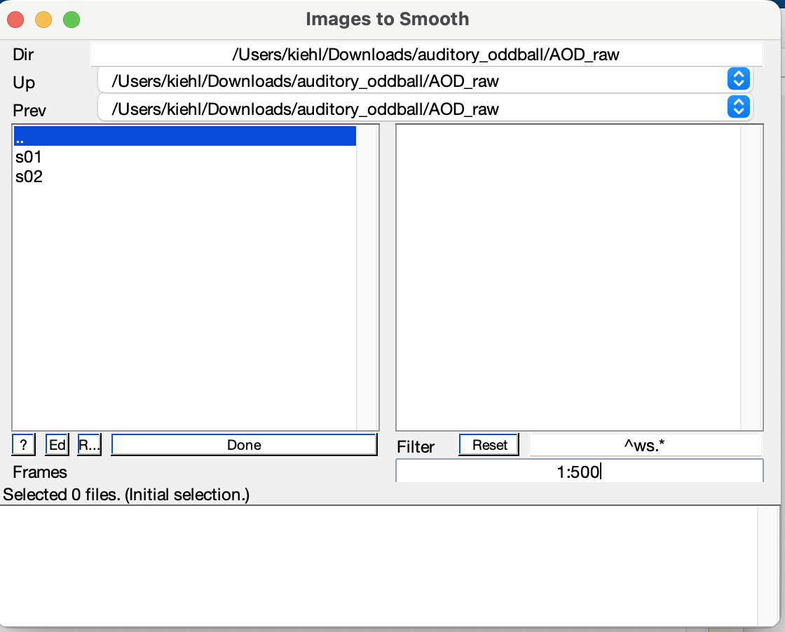
Click Smooth; under Images to Smooth click Specify, filter ^ws.* with frames 1:500, and use the recursive (R) button from AOD_raw to collect all runs.
Keep FWHM at [8 8 8], click Done, then click the green Run icon; output images are prefixed sw.

Cheat sheet: normalization — full cheat sheet

Mind fMRI Image Acquisition and Analyses Course - Cheat Sheet for Normalization

-Spatial normalization –

This procedure takes the mean fMRI (EPI) image for each session for each subject and spatially normalizes (using linear and nonlinear (tailored basis set) to the EPI template provided with SPM. This latter procedure works well to account for EPI distortions and nonlinear warping that is not well managed if you use the alternative path of using the linear coregistration of the mean fMRI (EPI image) for each session for each subject to the subjects T1 (anatomical) images. Then the subject’s anatomical T1 image is used to determine spatial normalization parameters and these parameters are applied to the EPI images for that subject’s sessions since they are ‘coregistered’ to the subjects T1 data. This latter step does not consider the nonlinearities inherent in EPI data.

Here is the citation relevant to this process:

Calhoun, V.D., Wager, T.D., Krishnan, A., Rosch, K.S., Seymour, K.E., Nebel, M.B., Mostofsky, S.H., Nyalakanai, P., & Kiehl, K.A. (2017). The impact of T1 vs EPI spatial registration templates for fMRI. Human Brain Mapping, 38(11), 5331-5342. PMID: 28745021 PMCID: PMC5565844 DOI: 10.1002/hbm.23737

- Set your working directory:

- click on ‘utils’ on the spm gui

- select ‘cd’ – dialog box opens, select your working directory (e.g., c:\mind)

- Start normalization –

- click on ‘normalization’ button in spm gui; select ‘normalize <-X’

- in the spm graphics gui, select ‘New “Normalize: Estimate & Write”

We are going to use the ‘old normalize routine’.

Using your mouse, right click in the ‘module list’ and delete the Normalize process.

Then select the SPM button, tools, old normalize, estimate and write.

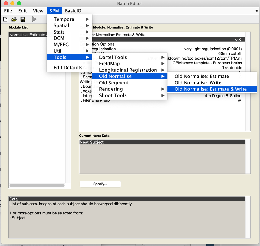
Graphical user interface, text, application Description automatically generated

- click on ‘+Normalize: Estimate & Write’ to expand to see:

-Normalize: Estimate & Write

Data <. X

+Estimation Options

+Writing Options

-Click on ‘Data <-X’

-Click on ‘New “Subject”’ 4 times (once for each session x 2 subjects)

Your display should now look like:

-Normalize: Estimate & Write

Data

+Subject <-X

+Subject <-X

+Subject <-X

+Subject <-X

+Estimation Options

+Write Options

Now you can click on the first ‘Subject <-X’ above
Then click on ‘Source Image <-X’
- Select ‘specify files’
- Select directory ‘c:\mind\data\auditory_oddball\AOD_raw\s01\01’
  - Select the mean EPI image for this subject.
    - means01_aod_run1.nii

Select ‘Images to write <-X

- Select directory ‘c:\mind\data\auditory_oddball\AOD_raw\s01\run1’

use the filter settings [1:200] in the window to help you select the right scans
- Right click on mouse and ‘select all’ images
  - s01_aod_run1.nii,1 to s01_aod_run1.nii,189’

Repeat ‘subject’ specification three more times to select the mean image for s01 run2, s02 run1, and s02 run2. carefully selecting the mean image and corresponding functional images to normalize for each session.

Click on ‘estimation options’,

select ‘template image <-X’
- specify files – go to c:\mind\toolboxes\spm12\toolbox\OldNorm\’ and select the ‘EPI.nii’ image.
All other options are set for you by default. Always review the spm normalization postscript output to ensure that you have used ‘4x5x4 basis functions’. If you see ‘9x12x9’ then you may need to renormalize the data and set the ‘nonlinear frequency cutoff to 45’.
Click on writing options if you want to change any other options. In our defaults, we are reslicing into 3x3x3 mm.

Click Run and spatial normalization will go.

The outputs include appending the spm_2022mar8.ps with the spatial normalization output files; you will see ‘means01_aod_run1_sn.mat’ – a file that contains the transformation data for native space to MNI space; and you will see ‘ws01_aod_run1.nii’ image file – this file contains the warped images that are now in MNI space.

Cheat sheet: spatial smoothing — full cheat sheet

Spatial smoothing:

Fire up spm gui. Click on the ‘Smooth’ button and it will populate the batch window.

A screenshot of a computer Description automatically generated

Click on the ‘specify’ button to select all the images you want to smooth.

You should select the ‘warped/subject’ images. So select ‘^ws.*’ and then 1:500 in each s01/run1 and s01/run2 directory. For the class we used the default of 8x8x8 smoothing. In practice, 2-3 times the original voxel size is rule-of-thumb.