Day 1 · Acquisition, preprocessing, and the GLM

Day 1Session 1.9Wager0:30 hHands-on session

CANlab interactive tools: basic analysis and visualization

A short walkthrough of the CANlab object-oriented tools using a MATLAB live script: load a set of first-level contrast images, check them for outliers, run a one-sample t-test with FDR thresholding, and visualize the results as slice montages, labeled region tables, and surface renderings. Shows how a full group analysis can be a handful of commands on a data object.

Take-aways

  • With the CANlab tools a group t-test, thresholding, and visualization take a few lines: load_image_set, ttest, threshold, montage, region, table.
  • Always run plot(img_obj) first; the outlier report can flag problem participants before you test.
  • Region tables and surface renderings are customizable objects, not static pictures.

Key terms

  • fmri_data object
  • load_image_set
  • statistic_image
  • ttest
  • threshold (FDR, extent k)
  • montage
  • region object
  • table (atlas labels)
  • surface
  • addbrain

Outline

What the session covers

01Setting up the tools

  • You need the CanlabCore and Neuroimaging_Pattern_Masks repositories from GitHub (see canlab.github.io/setup).
  • Add each with subfolders: cd to the repository, g = genpath(pwd); addpath(g); then savepath.
  • The script follows the CANlab walkthrough; more examples are at canlab.github.io/walkthroughs.
02Loading and inspecting data

  • img_obj = load_image_set('emotionreg') loads 30 contrast images (reappraise versus look negative) from Wager et al. 2008 into an fmri_data object.
  • plot(img_obj) shows the images, runs an outlier analysis (global mean, global mean to variance, spatial MAD, missing values, Mahalanobis distance), and opens spm_check_registration.
  • The outlier table reports counts per criterion, uncorrected and Bonferroni corrected; one image is flagged as a likely outlier with whole-brain deactivation.

03Running and thresholding the t-test

  • t = ttest(img_obj) runs a one-sample t-test across images and returns a statistic_image object.
  • t = threshold(t, .05, 'fdr', 'k', 10) applies FDR q < 0.05 with an extent threshold of 10 contiguous voxels.
  • Output reports the FDR p threshold (0.003 here), number of clusters (9), and positive and negative voxel counts.

04Showing results

  • montage(t) draws sagittal and axial slice montages of the thresholded map.
  • r = region(t) converts the map into a region object with one element per contiguous cluster.
  • table(r) prints a table with volume, peak XYZ, max Z, and automatic labels from the CANlab_2018_combined atlas, with atlas references.
  • Columns such as Perc_covered_by_label and Atlas_regions_covered tell you how well a cluster matches a single atlas region.

05Surface plots and customization

  • surface(t) renders the map on a cortical surface; surface(t, 'foursurfaces') and surface(t, 'coronal_slabs') give alternative views.
  • addbrain('midbrain_group') and addbrain('hires left') build custom surface sets whose FaceColor and FaceAlpha you can set.
  • surface(t, 'surface_handles', handles) renders blobs on those custom surfaces; help t.surface lists options.
  • The toolkit uses MATLAB handle graphics, so run the code line by line to see what each step does.
Axial brain slices in a false-color map — Lecture 1.3 slides (Wager)

Hands-on

Step by step

The walk-through below is distilled from the course cheat sheets. Data paths refer to the course Dropbox folder (e.g. data/auditory_oddball).

  1. Clone CanlabCore and Neuroimaging_Pattern_Masks from github.com/canlab if not already installed.
  2. In MATLAB, cd to each repository, run g = genpath(pwd); addpath(g); then savepath.
  3. img_obj = load_image_set('emotionreg'); to load the 30 emotion-regulation contrast images.
  4. plot(img_obj) and review the outlier analysis and registration check.
  5. t = ttest(img_obj); to run the one-sample t-test.
  6. t = threshold(t, .05, 'fdr', 'k', 10); to threshold at FDR q < .05 with 10-voxel extent.
  7. figure; axis off; montage(t); to view slice montages.
  8. r = region(t); table(r); to list clusters with atlas labels.
  9. surface(t); then try surface(t, 'foursurfaces') and surface(t, 'coronal_slabs').
  10. Build custom surfaces with handles = addbrain('midbrain_group'); handles = [handles addbrain('hires left')]; set(handles, 'FaceColor', [1 .5 .7], 'FaceAlpha', 1); surface(t, 'surface_handles', handles).

Basic t-test demo with CANlab tools (MATLAB live script)

From the instructors' research

Related figures

Examples of these concepts in published work by the course instructors.

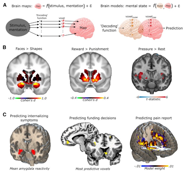
Encoding/decoding models and brain maps for faces, reward and pressure
Encoding/decoding models and brain maps for faces, reward and pressure. Kragel et al. (2018), Neuron
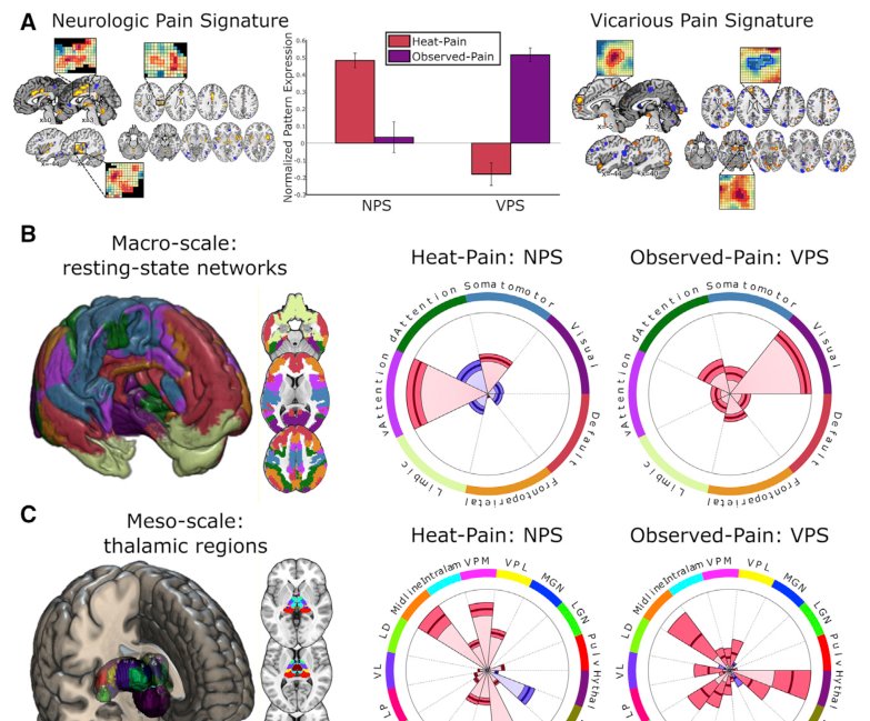
Neurologic Pain Signature vs vicarious pain signature across networks and thalamus
Neurologic Pain Signature vs vicarious pain signature across networks and thalamus. Kragel et al. (2018), Neuron