Day 1 · Acquisition, preprocessing, and the GLM

Day 1Session 1.3Wager0:10 hHands-on session

MATLAB basics and orientation

A brief tour of MATLAB for people who will use SPM: the desktop, getting help, variable types, scripts versus functions, and file types. Then orients you to how SPM works as a collection of functions that read and write image files, what NIfTI and MNI space mean, and which SPM defaults are worth changing before you start.

Take-aways

  • MATLAB scripts run in your workspace; functions are isolated black boxes; SPM is mostly functions that read and write image files.
  • Know where your images are in space: NIfTI headers, an origin near the anterior commissure, and MNI versus Talairach.
  • Set your own SPM defaults (high-pass filter, autocorrelation model, mask threshold, memory) in spm_my_defaults.m rather than accepting the stock values.

Key terms

  • Command Window
  • workspace
  • struct
  • cell array
  • script vs. function
  • .mat / .m / .mex
  • NIfTI
  • MNI space
  • spm_defaults.m
  • mask.nii
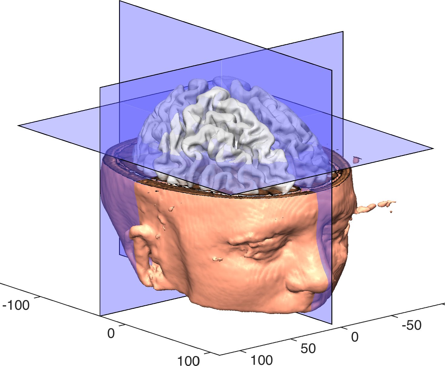
3-D head rendering with orthogonal slice planes
3-D head rendering with orthogonal slice planes. Lecture 1.3 slides (Wager)

Outline

What the session covers

01The MATLAB desktop and getting help

  • MATLAB's strengths for fMRI: visualization, matrix operations, and built-in help.
  • Desktop panels: Command Window, Command History, Workspace, and Current Directory.
  • Unix-style navigation: cd some_dir changes directory, ls lists files.
  • help spline prints a function's help text; helpdesk opens the Help Browser.
02Variables, types, and the workspace

  • Assignments like a = 5; b = 7; c = a + b create variables in the base workspace.
  • Types: double (numbers), char (text), struct (named fields, e.g., subj.id and subj.name), [ ] matrices, { } cell arrays of mixed content.
  • A struct can hold a region name, a time series vector, and a 3D coordinate grid together.
  • save mywkspace writes variables to a .mat file; load brings them back.
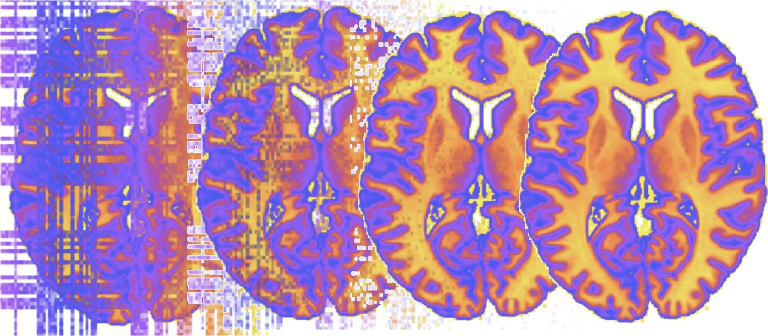
Axial brain slices in a false-color map
Axial brain slices in a false-color map. Lecture 1.3 slides (Wager)
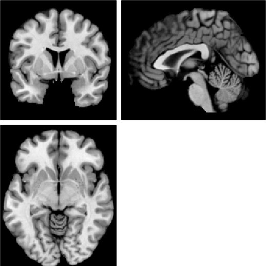
Coronal, sagittal, and axial anatomical slices
Coronal, sagittal, and axial anatomical slices. Lecture 1.3 slides (Wager)

03File types, scripts, and functions

  • .mat holds data; .m is an editable script or function; .mex is a compiled function you cannot edit.
  • A script is a list of commands run in the base workspace, as if typed.
  • A function has its own isolated workspace and sees only what is passed in: a black box with inputs and outputs.

04SPM as functions and files

  • SPM is a collection of functions: some open a GUI, a few return output to the workspace, most read and write files to disk.
  • Image formats: NIfTI (.nii); Analyze (.img, .hdr, plus a .mat in SPM); others outside SPM include CIFTI, GIFTI, and AFNI BRIK.
  • The origin [0 0 0] is typically the anterior commissure; MNI space is more precise than Talairach, though the SPM/FSL origin is slightly off the AC.
  • If which spm reports not found, use pathtool to add the SPM folder; which spm then shows the file being used.
  • Command-line entry points: spm_vol (header info), spm_read_vols (read data), spm_image('init', filename) (display in orthviews), spm_orthviews (control the display).

05SPM defaults worth changing

  • Defaults live in spm_defaults.m; put your overrides in spm_my_defaults.m on the path.
  • Recommended: defaults.stats.fmri.hpf = 180 (128 can be too low; choose deliberately) and defaults.stats.fmri.cvi = 'None' rather than AR(1) or FAST.
  • defaults.mask.thresh = -Inf instead of 0.8, so implicit masking does not block explicit masks.
  • defaults.stats.maxmem = 2^33 (about 8.6 GB) depending on your RAM; defaults.stats.topoFDR = 0.
  • Every SPM analysis writes mask.nii; a voxel missing in one subject is dropped for the whole group, whereas CANlab tools analyze available subjects voxel-wise.
Three axial slices with simulated effect patterns — Lecture 1.8 slides (Wager)

Hands-on

Step by step

The walk-through below is distilled from the course cheat sheets. Data paths refer to the course Dropbox folder (e.g. data/auditory_oddball).

  1. Open MATLAB and identify the Command Window, Command History, Workspace, and Current Directory panels.
  2. Use cd and ls to move to the mind folder and list its contents.
  3. Type help spline and helpdesk to see the two forms of help.
  4. Create variables: a = 5; name = 'Tor'; subj.id = 100; c = [1 2 3; 4 5 6; 7 8 9]; a cell array with { }.
  5. Save the workspace with save mywkspace, clear, and reload with load.
  6. Type which spm; if not found, use pathtool to add the SPM folder.
  7. Try spm_vol and spm_read_vols on a course image, then spm_image('init', filename) to view it.
  8. Review spm_defaults.m and create spm_my_defaults.m with the recommended hpf, cvi, mask.thresh, maxmem, and topoFDR settings.

From the instructors' research

Related figures

Examples of these concepts in published work by the course instructors.

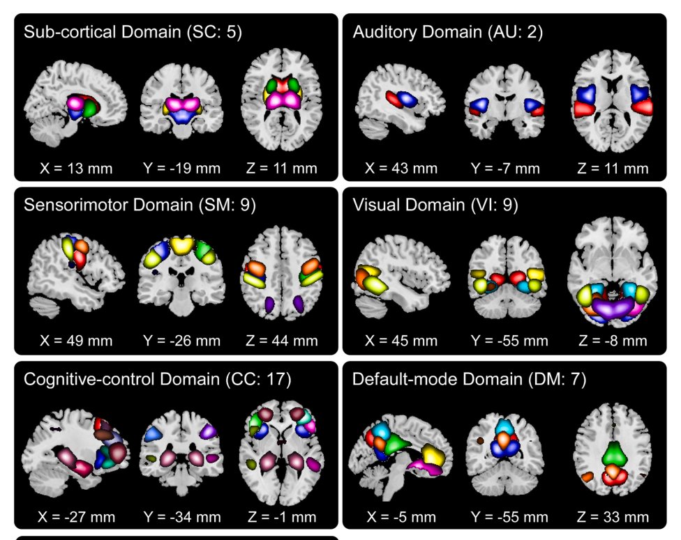
NeuroMark network templates by functional domain
NeuroMark network templates by functional domain. Du et al. (2020), NeuroImage: Clinical
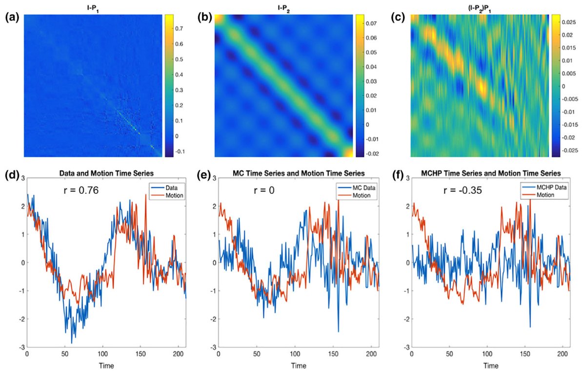
Projection matrices and motion-correlated time series across pipelines
Projection matrices and motion-correlated time series across pipelines. Lindquist et al. (2019), Human Brain Mapping