Day 1 · Acquisition, preprocessing, and the GLM

Day 1Session 1.6Kiehl1:00 hHands-on session

Spatial preprocessing: realignment, slice timing, unwarp

Explains why head motion is the dominant artifact in fMRI, how much motion is enough to matter, and the four lines of defense: prevention, detection and discarding, prospective correction, and post-processing realignment. Also covers physiological artifacts, movement-by-inhomogeneity interactions addressed by Unwarp, slice acquisition order, and the slice-timing problem. The hands-on part runs realignment with INRIAlign on the auditory oddball data.

Scroll down

Take-aways

Sub-millimeter motion produces signal changes as large as BOLD, especially at edges, so prevention and detection come before correction.
Realignment estimates six parameters per volume; prefer a robust cost function (INRIAlign) so real activation is not regressed away as motion.
Distortion changes with head position (Unwarp) and slices are acquired at different times (slice timing); both matter less with fast multiband acquisitions.

Key terms

rigid-body realignment
six motion parameters
INRIAlign
ART / composite motion
prospective motion correction
interpolation
physiological noise
movement-by-inhomogeneity interaction
Unwarp
slice-timing correction

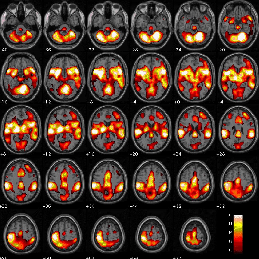
**Axial montage of group activation maps.** Lecture 1.6 slides (Kiehl)

Outline

What the session covers

01How much motion matters

Signal change from motion depends on how far the head moves and how sharp the local intensity edge is.
Inside the brain intensity varies only 10 to 20 percent, so a quarter-voxel shift (about 1 mm) gives a 3 to 5 percent change, BOLD-sized.
At the edge intensity varies 70 to 90 percent, so 1/20 of a voxel (about 187 microns) produces the same 3 to 5 percent change.
Most motion is random or slow drift and not task-correlated, so it rarely creates false activations, but it reduces sensitivity, especially near edges.
BOLD activity itself can sometimes be estimated as motion by the realignment algorithm.

02Prevention, detection, and prospective correction

Prevention: foam padding (not painfully tight) or bite bars; short TR, thin slices, sagittal acquisition; short runs and total scan time under about an hour.
Event-related designs are less vulnerable than blocked designs to motion that co-varies with task blocks.
Detection: know when motion occurred so you can log it, discard, or reacquire; real-time imaging allows this during the scan.
Prospective correction (Mayo group ONAV navigators; Lee et al. 1996, Ward et al. 2000) updates gradients each TR so acquisition tracks the head.

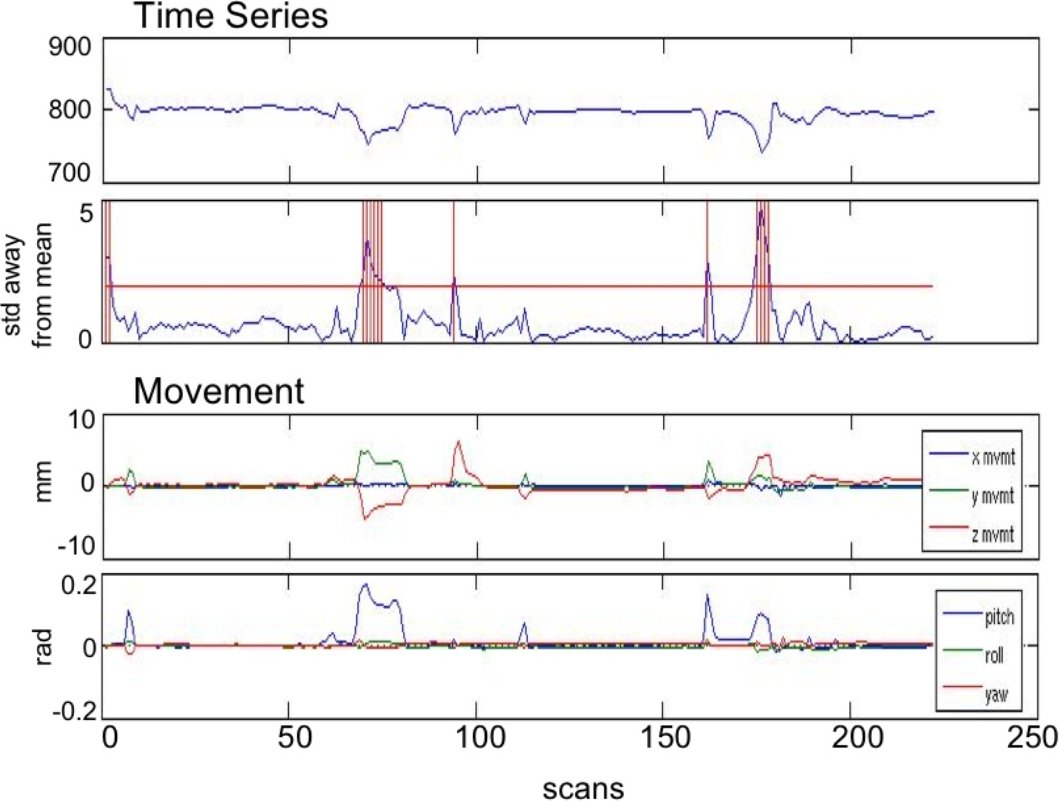
**Artifact detection: time series and motion traces.** Lecture 1.6 slides (Kiehl)

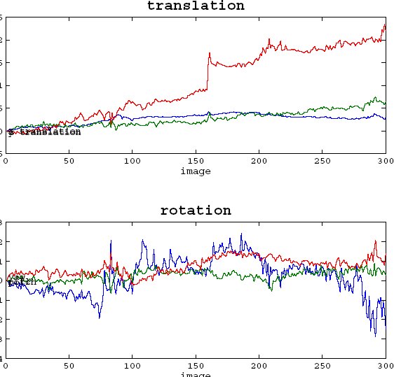
**Realignment translation and rotation estimates.** Lecture 1.6 slides (Kiehl)

03Quality assurance with ART

Review data bottom-up: check behavior (especially clinical groups), create a mean functional image, and watch the time series as a movie.
ART plots movement in mm and radians, global mean, and standard deviations from the mean, and flags motion outliers, intensity outliers, and combined outliers.
Composite motion converts the six parameters into trajectories of six bounding-box points and takes the maximum scan-to-scan displacement.
ART saves regressor files (art_regression_outliers_*.mat, art_regression_outliers_and_movement_*.mat) and a new analysis mask; thresholds can be changed and re-saved.

04Realignment: estimation and correction

The target is usually the first image of each run (if it looks fine); every later image is registered to it through hidden iterations.
Six rigid-body parameters are estimated: three translations (x, y, z) and three rotations.
Cost functions: mean squared difference (AIR, SPM) can regress away real signal; INRIAlign (Freire and Mangin 2001) is robust to local changes and eye movements.
Correction resamples the images using the estimated parameters; interpolation options include linear, bicubic, Fourier, and chirp-z.
Multiband data (TR 460 ms) and conventional EPI (TR 2000 ms) give parameter plots at very different temporal resolutions.

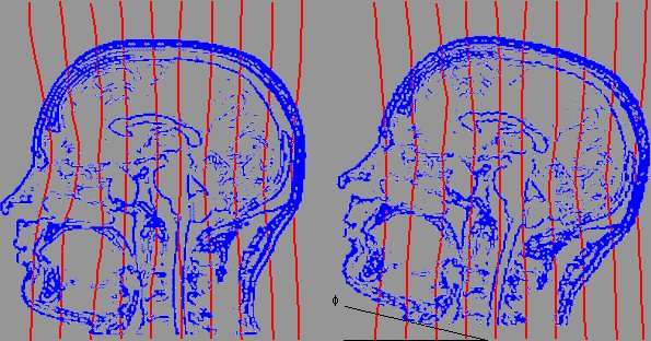
**Head contour overlays before and after coregistration.** Lecture 1.6 slides (Kiehl)

05Physiological artifacts and Unwarp

Respiration causes oscillations in signal through both motion and changes in the B0 field; iterative subtraction movies (i1 minus i2, i2 minus i3) reveal them.
Solutions: filtering, prospective or retrospective gating, and fast multiband TR (0.4 s) that separates cardiac and respiratory spectra (Tong and Frederick 2014).
After realignment, residual variance remains from movement-by-inhomogeneity interactions: the distortion field changes with head position.
Options: acquire a field map at every time point (about 50 percent slower) or run Andersson's Unwarp afterward, which is CPU intensive.
Susceptibility summary: prevent with thin slices, short TE, shimming; sequences with z-shim or tailored RF; post-process with unwarping; prefer event-related designs.

06Slice acquisition and slice timing

Slices are acquired one at a time (2D imaging), interleaved or sequential; sequential needs a small gap, but effective slice thickness is the same.
After 3D head motion the slices are no longer parallel to the brain; spatio-temporal blurring occurs with sequential order and is compounded by interleaving.
Adjacent slices are about 70 ms apart in sequential order but 1 to 2 s apart in interleaved order.
Slice-timing problem (Henson et al. 1999): one model for all slices gives different results with a canonical HRF depending on the reference slice.
Solutions: temporal interpolation (adds error, worse at long TR) or fast TRs plus a derivative boost (Calhoun et al. 2004); largely moot with multiband EPI.

Five dynamic connectivity states rendered on cortical surfaces — Rashid et al. (2014), Frontiers in Human Neuroscience

Hands-on

Step by step

The walk-through below is distilled from the course cheat sheets. Data paths refer to the course Dropbox folder (e.g. data/auditory_oddball).

In the SPM GUI click Utils > cd and set the working directory to c:\mind.
Click Toolboxes > INRIAlign; when asked to check local parameters, choose use defaults.
Enter number of subjects = 4 (2 subjects x 2 sessions).
For s01 run1: go to c:\mind\data\auditory_oddball\AOD_raw\s01\run1, filter [1:200], right-click Select All (s01_aod_run1.nii,1 to 189), Done.
Repeat for s01\run2 (s01_aod_run2.nii), s02\run1 (s02_aod_run1.nii), and s02\run2 (s02_aod_run2.nii).
Which option: coregister and reslice.
Reslice interpolation method: sinc.
Create what: mean image only.
Let INRIAlign run; check outputs rp_s01_aod_run1.txt (3 translations, 3 rotations), the motion plots in the spm_*.ps file, and means01_aod_run1.nii for each run.

Cheat sheet: realignment (INRIAlign) — full cheat sheet

Mind fMRI Image Acquisition and Analyses Course - Cheat Sheet for Course Realignment

-Realignment – using INRIAlign –

Freire, L. & Mangin, J.-F. (2001). Motion correction algorithms may

create spurious brain activations in the absence of subject motion.

NeuroImage, vol. 14, pp. 709–722.

See also:

Freire, L., Roche, A. & Mangin, J.-F. (2002). What is the best similarity measure for motion correction in fMRI time series? IEEE Transactions on Medical Imaging, 21 (5), 470-484.

– INRIAlign.

- Set your working directory:

- click on ‘utils’ on the spm gui

- select ‘cd’ – dialog box opens, select your working directory (e.g., c:\mind)

- Start realignment – INRIAlign version –

‘select ‘toolboxes’ on the bottom left spm gui. Select ‘INRIAlign’.

a dialog box is generated that asks to ‘check local parameters’.
You may ‘use defaults’.
- Number of subjects ‘select 4’ (2 subjects x 2 sessions)
- The file select dialog box will open
- Select directory ‘c:\mind\data\auditory_oddball\AOD_raw\s01\run1’
- use the filter settings [1:200] in the window to help you select the right scans
  - Right click on mouse and ‘select all’ images
    - s01_aod_run1.nii,1 to s01_aod_run1.nii,189’
CLICK on ‘DONE’ to complete files for first subject.
- Select data for subject 1 session 2- directory ‘c:\mind\data\auditory_oddball\AOD_raw\s01\run2’
- use the filter settings [1:200] in the window to help you select the right scans
  - Right click on mouse and ‘select all’ images
    - s01_aod_run2.nii,1 to s01_aod_run2.nii,189’
CLICK on ‘DONE’ to complete files for second subject (session 2 of s01) .
- Select data for subject 2 session 1 - directory ‘c:\mind\data\auditory_oddball\AOD_raw\s02\run1’
- use the filter settings [1:200] in the window to help you select the right scans
  - Right click on mouse and ‘select all’ images
    - s02_aod_run1.nii,1 to s02_aod_run1.nii,189’

- CLICK on ‘DONE’ to complete files for third subject (session 1 of subject s02).

Select data for subject 2 session 2 - directory ‘c:\mind\data\auditory_oddball\AOD_raw\s02\run2’
use the filter settings [1:200] in the window to help you select the right scans
- Right click on mouse and ‘select all’ images
  - s02_aod_run2.nii,1 to s02_aod_run2.nii,189’

- CLICK on ‘DONE’ to complete files for third subject (session 2 of subject s02).

Under the dialog ‘Which Option?’

select ‘coregister and reslice’

Under dialog ‘Reslice interpolation method’

select ‘sync’

Under dialog ‘Create what?’

select ‘mean image only’

INRIAlign starts. Output maps are same as spm’s default realignment. The process will also output the realignment parameters (3 rotation x 3 translation) (rp_s01_aod_run1.txt), a postscript file with the motion plots (spm_2022Mar08.ps), and a mean image for each run (means01_aod_run1.nii).

Previous · 1.5Intro to SPM: data checking, reorienting data Next · 1.7Preprocessing: coregistration, normalization, smoothing